SpecMod tutorial

Fitting a source model to the spectra of a small induced earthquake, end to end.

The event is a Preston New Road induced earthquake of 2019-08-26, recorded on the LV and UR networks during hydraulic fracturing near Blackpool, UK. The waveforms and station metadata are committed with the package (224 KB), so this notebook needs no network access.

Five stages, one section each:

1. Read and prepare the waveforms — geometry, picks, instrument response.

2. Cut a signal window and a noise window to judge it against.

3. Transform both to spectra and select the usable bandwidth.

4. Fit a source model over that bandwidth.

5. Save the results.

Every processing step is written down with its equation in docs/processing.md; this is the same pipeline with the numbers left in.

1. Read and prepare

from __future__ import annotations

from pathlib import Path

import matplotlib.pyplot as plt
import numpy as np
import pandas as pd
from obspy import UTCDateTime, read, read_inventory
from obspy.core.stream import Stream
from pandas.core.frame import DataFrame
from pandas.core.series import Series

import specmod.preprocess as pre
import specmod.utils as ut
from specmod.core.collection import SpectrumPair, SpectrumSet
from specmod.pipeline import spectrum_set_from_streams
from specmod.staged import StagedFit

# Relative to this notebook, so it runs from wherever it is opened.
EVENTS = Path("data/events")
EVENT = "2019-08-26T07:30:47.000000Z" # Event origin time
DATA: Path = EVENTS / EVENT
WAVEFORMS: Path = DATA / "waveforms"
STATIONS: Path = DATA / "stations" / "*.xml"
PICKS: Path = DATA / "picks"
OUTPUT: Path = DATA / "spectra"

The origin is what distances and theoretical arrivals are measured from.

The hypocentre and origin time here are the published catalogue’s, from the PNR-2 dataset released with Cuadrilla’s hydraulic-fracture monitoring. Its easting/northing are British National Grid, converted to WGS84; the catalogue gives depth as an elevation of -2040 m.

olat, olon, odep = 53.785021, -2.970780, 2.04
otime = UTCDateTime(EVENT)

# The two horizontal components. S-wave amplitudes are what the source model
# is fitted to, so the verticals are not read.
st = read(str(object=WAVEFORMS / "*HHE*"), format="mseed") + read(
    str(object=WAVEFORMS / "*HHN*"), format="mseed"
)
inv = read_inventory(str(object=STATIONS), "stationxml")
print(f"{len(st)} traces, {len({tr.stats.station for tr in st})} stations")

28 traces, 14 stations

# Source-receiver geometry, from the inventory. Adds repi, rhyp, azimuth and
# back-azimuth to every trace — on a new stream, which is why the result is
# assigned back. Nothing in `preprocess` modifies what it is given.
st = pre.with_distance(st, olat, olon, odep, otime, inventory=inv, dtype="mseed")

# P and S arrivals, from QuakeML. `with_picks` also reads Snuffler marker
# files, dispatching on the suffix.
st = pre.with_picks(st, next(PICKS.glob("*.xml")))

# A trace with no S pick cannot have an S window cut from it. Dropping them
# here is the pipeline's own idiom for "unusable".
st = Stream([tr for tr in st if "s_time" in tr.stats])

print(f"{len(st)} traces with both picks")

28 traces with both picks

/home/docs/checkouts/readthedocs.org/user_builds/specmod/envs/50/lib/python3.11/site-packages/obspy/core/inventory/network.py:321: UserWarning: Found more than one matching channel metadata. Returning first.
  warnings.warn(msg)

Instrument correction happens here, in the notebook, not inside the package. That is deliberate: the choice of output units and water level is part of the science, and burying it in a library call makes it invisible in the record of what was run.

Demeaning matters more than it looks. A non-zero mean puts all of its energy in the DC bin, which every estimator discards — so leaving it in loses energy that the Parseval check would report as a failure.

st.detrend("linear")
st.detrend("demean")
st.taper(0.05)
st.remove_response(inv, output="VEL")  # ground velocity, m/s

/home/docs/checkouts/readthedocs.org/user_builds/specmod/envs/50/lib/python3.11/site-packages/obspy/core/inventory/network.py:251: UserWarning: Found more than one matching response. Returning first.
  warnings.warn(msg)

28 Trace(s) in Stream:

LV.L001..HHE | 2019-08-26T07:30:46.900000Z - 2019-08-26T07:30:53.900000Z | 100.0 Hz, 701 samples
...
(26 other traces)
...
UR.AQ10.00.HHN | 2019-08-26T07:30:49.500000Z - 2019-08-26T07:30:56.500000Z | 100.0 Hz, 701 samples

[Use "print(Stream.__str__(extended=True))" to print all Traces]

ut.plot_traces(st=st.copy(), plot_theoreticals=True, conv=1)
plt.show()

2. Cut the windows

The S-window opens at a fixed fraction of the elapsed P–S time after the P arrival, then is refined onto the part of it that actually carries energy: the window is tightened to where the cumulative squared amplitude runs between its 1st and 99th percentiles. That is why these come out at 1.8–3.7 s rather than the nominal 20 s.

The noise window ends shortly before the P arrival and is asked for the same length as the refined signal window. It rarely gets it — see below.

sig: Stream = pre.s_window(
    st, rafp=0.8, tafs=20, time_after="absolute_time", refine_window=True
)
# `st` is untouched by the cut above, so the noise is measured from the same
# starting point rather than from an already-trimmed record.
noise: Stream = pre.get_noise_p(st, sig)

# Every noise window here is shorter than the signal it is judged against,
# because the records begin only ~2 s before the P arrival. This is normal and
# is corrected for; it is why `SpectrumPair` carries a resolution floor rather
# than assuming the two spectra share a frequency resolution.
for s, n in list(zip(sig, noise, strict=False))[:4]:
    asked = float(n.stats["wend_requested"] - n.stats["wstart_requested"])
    got = float(n.stats["wend"] - n.stats["wstart"])
    print(
        f"{s.id:16s} signal {s.stats.endtime - s.stats.starttime:5.2f} s   "
        f"noise asked {asked:5.2f} s, got {got:5.2f} s"
    )

LV.L001..HHE     signal  3.04 s   noise asked  3.04 s, got  1.63 s
LV.L002..HHE     signal  3.34 s   noise asked  3.34 s, got  1.51 s
LV.L006..HHE     signal  2.90 s   noise asked  2.90 s, got  1.42 s
LV.L007..HHE     signal  2.79 s   noise asked  2.79 s, got  1.48 s

ut.plot_traces(st=st.copy(), plot_windows=True, conv=1, sig=sig, noise=noise)
plt.show()

3. Spectra and bandwidth

from specmod.core.collection import SpectrumSet
from specmod.pipeline import
spectrum_set_from_streams

spectrum_set_from_streams transforms both windows, puts the noise on the signal’s frequency axis, bins both, raises the noise to account for what sits under the signal, takes the ratio and selects the band where it passes.

Which estimator is used is configuration, not code: fft, welch, multitaper, quadratic and cwt all satisfy the same Parseval contract, so they are interchangeable here. The shipped default is multitaper.

spectra: SpectrumSet = spectrum_set_from_streams(signal=sig, noise=noise)
print(f"{len(spectra)} spectra for event {spectra.event}")
print(
    f"{sum(p.passes for p in spectra.pairs.values())} passed the signal-to-noise gate"
)

28 spectra for event 2019-08-26T07:30:47.000000Z
28 passed the signal-to-noise gate

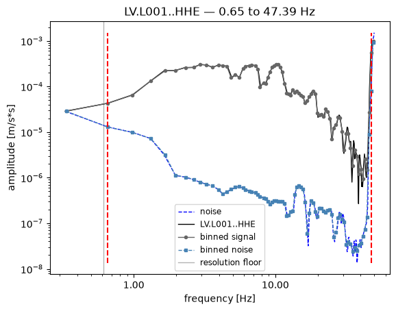
# One station in detail: signal, noise, the binned spectra the ratio is
# actually computed on, the selected band (red) and the resolution floor (grey).
from specmod.plotting import plot_pair, plot_set

station: str = spectra.ids()[0]
plot_pair(pair=spectra[station], id=station, show_binned=True)
plt.show()

pair: SpectrumPair = spectra[station]
if pair.band is not None:
    print(f"band             {pair.band[0]:.2f} to {pair.band[1]:.2f} Hz")
else:
    print("band            unavailable")
print(f"resolution floor {pair.resolution_floor:.2f} Hz  (the shorter window's 1/T)")
print(f"units            {pair.signal.unit}")

band             0.65 to 47.39 Hz
resolution floor 0.61 Hz  (the shorter window's 1/T)
units            m/s*s

The band is a choice, and the automatic one runs high

Both automatic selectors walk outward from where the ratio is best and stop where it falls below the threshold. Nothing in that walk knows about the instrument. Approaching Nyquist the signal and the noise roll off into the anti-alias filter together, so their ratio can stay above the threshold through a region where neither carries usable information — and the walk runs on until it hits the end of the array.

Here is where the high edges of this event actually land, as a fraction of each trace’s own Nyquist frequency:

import numpy as np


def band_report(spectra: SpectrumSet) -> "pd.DataFrame":
    rows = []
    for id in spectra.ids():
        p = spectra[id]
        if p.band is None:
            continue
        nyquist = p.signal.sampling_rate / 2
        rows.append(
            {
                "id": id,
                "low": p.band[0],
                "high": p.band[1],
                "nyquist": nyquist,
                "of_nyquist": p.band[1] / nyquist,
            }
        )
    return pd.DataFrame(rows).set_index("id")


report = band_report(spectra)
print(f"median high edge: {report.of_nyquist.median():.0%} of Nyquist")
for level in (0.5, 0.8, 0.9):
    print(f"  above {level:.0%}: {(report.of_nyquist > level).sum():2d} of {len(report)}")
report.sort_values("of_nyquist", ascending=False).head(5).round(2)

median high edge: 78% of Nyquist
  above 50%: 21 of 28
  above 80%: 11 of 28
  above 90%:  5 of 28

	low	high	nyquist	of_nyquist
id
UR.AQ09.00.HHE	0.66	47.56	50.0	0.95
LV.L001..HHN	1.12	47.54	50.0	0.95
UR.AQ09.00.HHN	0.67	47.40	50.0	0.95
LV.L001..HHE	0.65	47.39	50.0	0.95
LV.L009..HHE	0.68	45.74	50.0	0.91

The stations at the top of that table are having their anti-alias filter fitted as though it were a source spectrum. There are three ways to take control of it, and they are not interchangeable.

One — raise the signal-to-noise threshold. The bluntest and often the right one: it demands more evidence everywhere, so the walk stops earlier. It is global, it tightens the low edge as well, and pushed far enough it starts rejecting stations outright — which may be what you want, or may be throwing away the quiet stations that carry the long-period plateau.

thresholds = (3.0, 5.0, 10.0, 20.0, 50.0)
rows = []
for t in thresholds:
    trial = spectrum_set_from_streams(signal=sig, noise=noise, compare={"threshold": t})
    r = band_report(trial)
    rows.append(
        {
            "threshold": t,
            "with a band": len(r),
            "median high (Hz)": r.high.median(),
            "median % Nyquist": r.of_nyquist.median(),
            "above 80%": int((r.of_nyquist > 0.8).sum()),
        }
    )
pd.DataFrame(rows).set_index("threshold").round(3)

	with a band	median high (Hz)	median % Nyquist	above 80%
threshold
3.0	28	43.727	0.777	11
5.0	28	42.493	0.682	9
10.0	28	32.162	0.534	6
20.0	28	23.674	0.384	5
50.0	25	14.637	0.259	1

Note the first column: past a point the threshold buys a tighter band by losing stations, and a station that drops out contributes nothing to the event average at all.

Two — cap the high edge. max_nyquist_fraction clamps whatever the selector returned, so the automatic choice still does the work and only the part that overran is refused. It is a fraction rather than a frequency because this network records at two different rates, and the roll-off it guards against moves with the rate.

It is applied after selection, so it constrains every strategy the same way — it is a statement about the recording, not about how the band was picked.

capped = spectrum_set_from_streams(
    signal=sig, noise=noise, compare={"max_nyquist_fraction": 0.8}
)

before, after = band_report(spectra), band_report(capped)
moved = (before.high - after.high).abs() > 1e-9
print(f"bands changed: {int(moved.sum())} of {len(before)}")
print(f"median high edge: {before.high.median():.1f} Hz -> {after.high.median():.1f} Hz")

# Imported here rather than at the top: section 4 is where fitting is
# introduced, and this section only needs it to show what the band costs.
from specmod.fitting import FitSpectra

fits_before = FitSpectra(spectra)
fits_before.fit_spectra()
fits_after = FitSpectra(capped)
fits_after.fit_spectra()
fc = (
    fits_before.table.set_index("id")[["fc"]]
    .join(fits_after.table.set_index("id")[["fc"]], lsuffix="_auto", rsuffix="_capped")
    .loc[moved[moved].index]
)
fc["change %"] = (fc.fc_capped - fc.fc_auto) / fc.fc_auto * 100
print(f"\nmedian |change| in fc on those: {fc['change %'].abs().median():.1f}%")
fc.reindex(fc["change %"].abs().sort_values(ascending=False).index).head(5).round(2)

bands changed: 11 of 28
median high edge: 43.7 Hz -> 40.0 Hz

median |change| in fc on those: 18.0%

	fc_auto	fc_capped	change %
id
LV.L001..HHN	2.98	11.26	277.30
LV.L001..HHE	4.39	8.97	104.19
UR.AQ04.00.HHE	6.36	11.13	75.14
LV.L009..HHE	4.32	2.84	-34.19
UR.AQ07.00.HHE	3.19	3.80	19.33

That is the number to take seriously. The band is not a presentational choice — moving it moves the fitted corner frequency by a median of over ten percent on the stations it touches, and by a factor of three on the worst. Stress drop scales as \(f_c^3\), so a factor of three in \(f_c\) is a factor of twenty-seven in stress drop.

It does not follow that the capped answer is the right one. What follows is that this is a decision, it was being made silently by a default, and it has to be visible.

Three — say the band outright. For a study that fixes one band across every event so its results stay comparable, or for a single station whose automatic band you have looked at and rejected.

from specmod.core.bandwidth import FixedBandwidth

# Everything on one band, ignoring the ratio entirely. Configuration reaches
# this too, as `[snr] bandwidth_method = "fixed"` with `fixed_band = [1, 25]`.
imposed = spectrum_set_from_streams(
    signal=sig, noise=noise, compare={"bandwidth": FixedBandwidth(1.0, 25.0)}
)
print("fixed:  ", band_report(imposed).high.describe()[["min", "max"]].round(2).to_dict())

# Or correct exactly one station, leaving every other pair as it was. Returns
# a new pair; `spectra` is untouched.
one = spectra[station].with_band((1.0, 20.0))
print(f"{station}: {spectra[station].band[1]:.2f} Hz -> {one.band[1]:.2f} Hz")

# Either way the pair records that its band was asserted rather than measured,
# so a result read back later still knows the difference.
print("recorded as:", one.meta["band_imposed"], "|", imposed[station].meta["band_imposed"])

fixed:   {'min': 25.0, 'max': 25.0}
LV.L001..HHE: 47.39 Hz -> 20.00 Hz
recorded as: manual | fixed

Changing ground-motion domain

The response was removed to velocity, but a source model is often read on displacement. to_motion converts the whole event and returns a new set — the velocity one is untouched, so both exist at once.

displacement = spectra.to_motion("displacement")
print(f"velocity     {spectra[station].signal.unit}")
print(f"displacement {displacement[station].signal.unit}")

# The unbinned signal-to-noise ratio is invariant under this — both spectra are
# divided by the same 2*pi*f — but the *binned* ratio is not, because a bin
# holds a geometric mean. So a few bands do move.
moved = [i for i in spectra.ids() if spectra[i].band != displacement[i].band]
print(f"bands that moved: {len(moved)} of {len(spectra)}")

velocity     m/s*s
displacement m*s
bands that moved: 0 of 28

4. Fit a source model

The model comes from configuration — a Brune source with constant Q by default — and the initial guesses are derived from each spectrum: the plateau from the largest amplitude inside the band, the corner from where that maximum falls.

FitSpectra(spectra) then fit_spectra() is the whole thing. The minimiser (Powell), the t* lower bound and whether to fit the binned or unbinned spectrum all come from [fitting] in the configuration, so the defaults are recorded rather than remembered.

from specmod import sources
from specmod.fitting import FitSpectra, initial_guess

print(sources.from_config().describe())
guess = initial_guess(spectra)
print(f"guesses for {len(guess)} of {len(spectra)} stations")

brune+constant_q in velocity
guesses for 28 of 28 stations

fits = FitSpectra(spectra)
fits.fit_spectra()
print(
    f"{len(fits.models)} fitted, "
    f"{fits.table['pass_fitting'].sum()} passed the fit checks."
)

28 fitted, 28 passed the fit checks.

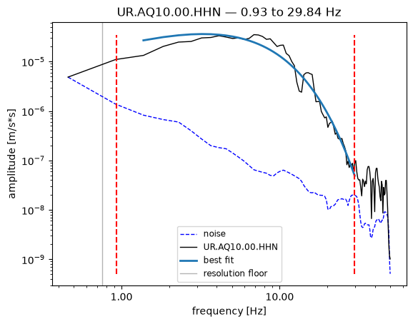
The guess is only a starting point, and a crude one: it takes the largest amplitude inside the band, which on a velocity spectrum is near the corner but can land at the band edge when the corner sits outside the resolvable range. Comparing it with where the fit ended up shows how much work the minimiser is doing.

fitted = fits.table.set_index("id")["fc"]
guessed_fc = {}
band_high = {}

for station, value in guess.items():
    guessed_fc[station] = (
        value["fc"] if isinstance(value, dict) and "fc" in value else None
    )

    band: tuple[float, float] | None = spectra[station].band
    band_high[station] = band[1] if band is not None else None

comparison = pd.DataFrame(
    {
        "guessed fc": guessed_fc,
        "fitted fc": fitted,
        "band high": band_high,
    }
).round(2)
comparison.head(8)

	guessed fc	fitted fc	band high
LV.L001..HHE	47.21	4.39	47.39
LV.L002..HHE	4.78	5.89	33.67
LV.L006..HHE	3.44	3.01	38.85
LV.L007..HHE	3.57	6.37	26.30
LV.L008..HHE	2.92	19.42	18.89
LV.L009..HHE	3.10	4.32	45.74
UR.AQ01.00.HHE	5.14	9.86	30.85
UR.AQ03.00.HHE	5.92	2.83	77.70

# The fitted model over the spectrum it was fitted to.
plot_pair(spectra[station], id=station, fit=fits.models[station])
plt.show()

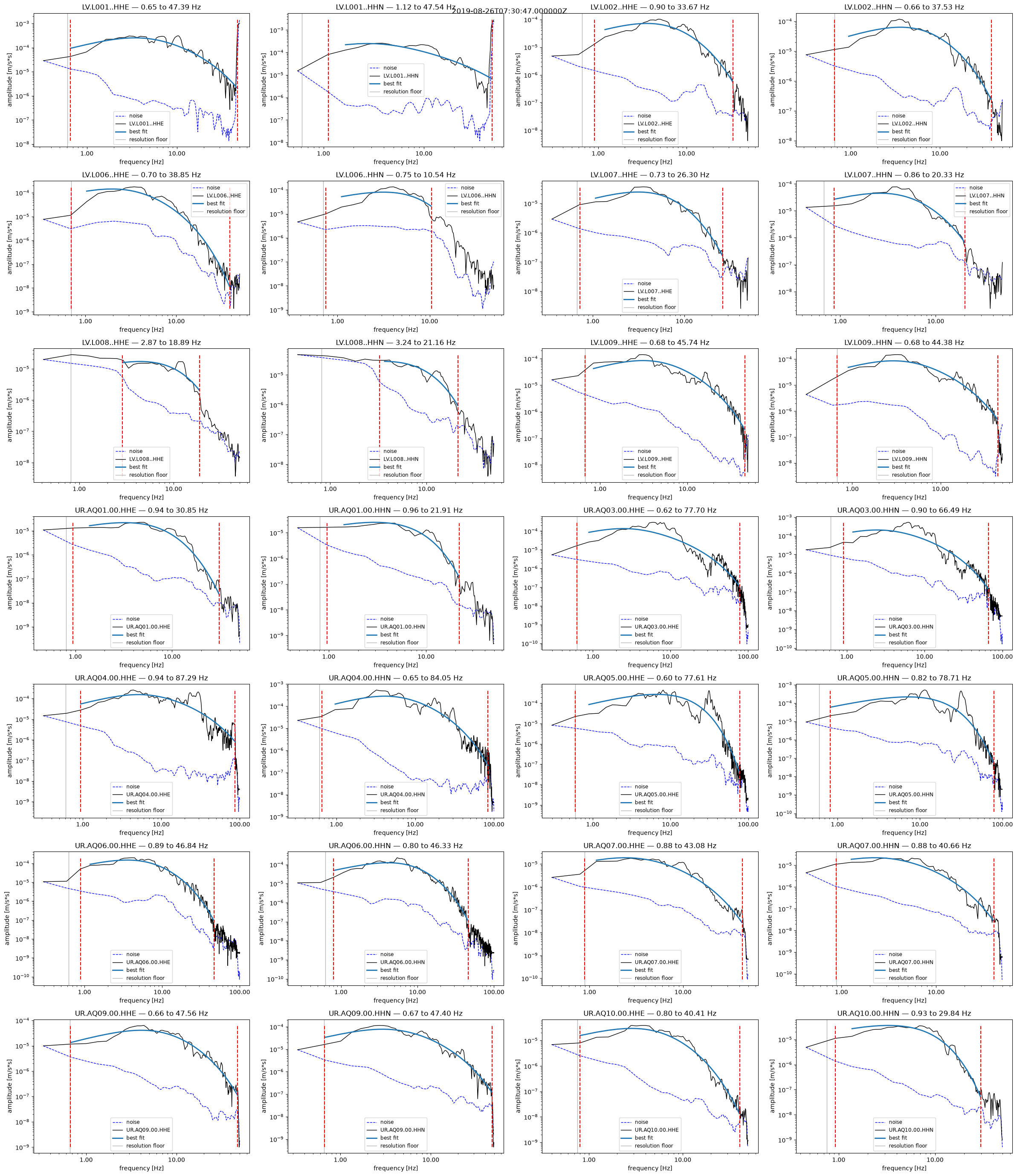
# Or the whole event at once.
plot_set(spectra, fits=fits, columns=4)
plt.show()

fits.table[["id", "fc", "fc-stderr", "llpsp", "ts", "pass_fitting"]].head(10)

	id	fc	fc-stderr	llpsp	ts	pass_fitting
0	LV.L001..HHE	4.394520	None	-4.614151	0.023064	True
1	LV.L002..HHE	5.888485	None	-5.154718	0.041821	True
2	LV.L006..HHE	3.007301	None	-4.601092	0.066537	True
3	LV.L007..HHE	6.368972	None	-5.546449	0.061823	True
4	LV.L008..HHE	19.418044	None	-5.793181	0.065783	True
5	LV.L009..HHE	4.322822	None	-5.045543	0.032677	True
6	UR.AQ01.00.HHE	9.862871	None	-5.573028	0.079704	True
7	UR.AQ03.00.HHE	2.834860	None	-4.749034	0.019050	True
8	UR.AQ04.00.HHE	6.356409	None	-5.009011	0.012962	True
9	UR.AQ05.00.HHE	59.638328	None	-4.759449	0.046850	True

The fit is not unique, and that is not a detail

fc-stderr is empty above. Powell — the shipped default, and what the published workflow used — searches without building a covariance matrix, so lmfit has no uncertainties to report. The obvious response is to use a method that does:

fits.fit_spectra(method="leastsq")

But the two do not merely differ in whether they report an error bar. They land on different answers, and comparing them is the most useful thing this notebook can show you, because it makes visible something a single fit hides: minimising misfit does not have one solution here, and choosing between the candidates is your job rather than the optimiser’s.

alternatives: dict[str, FitSpectra] = {}
for method in ("powell", "leastsq"):
    run = FitSpectra(spectra)
    run.fit_spectra(method=method)
    alternatives[method] = run

comparison = pd.DataFrame(
    data={
        "fc powell": alternatives["powell"].table.set_index(keys="id")["fc"],
        "fc leastsq": alternatives["leastsq"].table.set_index(keys="id")["fc"],
        "redchi powell": alternatives["powell"].table.set_index(keys="id")["redchi"],
        "redchi leastsq": alternatives["leastsq"].table.set_index(keys="id")["redchi"],
    }
)
comparison["fc ratio"] = comparison["fc leastsq"] / comparison["fc powell"]

# Ordered by how much the two disagree.
comparison.reindex(
    labels=(comparison["fc ratio"] - 1).abs().sort_values(ascending=False).index
).head(n=6).round(decimals=3)

	fc powell	fc leastsq	redchi powell	redchi leastsq	fc ratio
id
UR.AQ10.00.HHN	21.256	14.747	0.026	0.025	0.694
UR.AQ03.00.HHN	2.966	2.737	0.127	0.127	0.923
LV.L001..HHN	2.983	3.122	0.344	0.344	1.047
LV.L008..HHE	19.418	19.201	0.028	0.028	0.989
UR.AQ06.00.HHE	6.271	6.308	0.048	0.048	1.006
LV.L008..HHN	23.157	23.063	0.032	0.032	0.996

Most stations agree to a fraction of a percent. A few do not, and the top of that table is the interesting part: the two minimisers reach the same reduced chi-squared to within a few percent at corner frequencies that differ by tens of percent.

That matters more than the number suggests. Stress drop scales as \(f_c^3\), so a corner frequency ratio of 1.4 is a factor of three in stress drop — between two fits you cannot tell apart on goodness of fit alone.

worst = (comparison["fc ratio"] - 1).abs().idxmax()
row = comparison.loc[worst]
ratio = row["fc powell"] / row["fc leastsq"]
print(f"{worst}")
for method in ("powell", "leastsq"):
    print(
        f"  {method:8s} fc = {row['fc ' + method]:6.2f} Hz"
        f"   reduced chi-sq {row['redchi ' + method]:.4f}"
    )
print(f"  ratio in fc =  {ratio:.2f}")
print(f"  implied stress-drop ratio (fc^3)  {ratio**3:.2f}")

UR.AQ10.00.HHN
  powell   fc =  21.26 Hz   reduced chi-sq 0.0259
  leastsq  fc =  14.75 Hz   reduced chi-sq 0.0254
  ratio in fc =  1.44
  implied stress-drop ratio (fc^3)  2.99

# Both models over the spectrum they were fitted to.
worst_id = str(object=worst)
plot_pair(
    pair=spectra[worst_id],
    id=worst_id,
    fit={m: run.models[worst_id] for m, run in alternatives.items()},
)
plt.show()

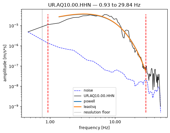
Look at where they differ: high up the falling limb, where the source corner and the attenuation \(t^*\) trade off against each other. Both curves pass through the data; they disagree about how much of the high-frequency falloff is the source rolling off and how much is the path absorbing. That trade-off is intrinsic to fitting \(\Omega\), \(f_c\) and \(t^*\) together from one spectrum, and no minimiser can resolve it — it needs either more information (several stations, a spectral ratio, an independent \(Q\)) or a decision.

So: fit both ways, look at the spread, and record which you chose. [fitting] method in the configuration is where that choice belongs, so that a run says what it did rather than relying on anyone’s memory.

pass_fitting marks a fit whose parameter is pinned against one of its bounds — the minimiser saying “further, if you would let me”, with the bound reported instead of a measurement. Without uncertainties the test is weaker, because it can only ask whether the value is the bound rather than whether it reaches one.

for method, run in alternatives.items():
    table: DataFrame = run.table
    print(
        f"{method:9s} {table['pass_fitting'].sum():2d}/{len(table)} passed"
        f"   uncertainties reported: {table['fc-stderr'].notna().sum()}/{len(table)}"
    )

powell    28/28 passed   uncertainties reported: 0/28
leastsq   22/28 passed   uncertainties reported: 28/28

Why the answer comes from many stations, and from two stages

The ambiguity above is a property of one spectrum, and that is the whole reason the method does not use one. \(f_c\) belongs to the source — every station is looking at the same rupture, so there is one value of it for the event. \(t^*\) belongs to the path, and every station has a different one.

So the trade-off that makes a single fit ambiguous does not point the same way twice. A station whose \(t^*\) is over-estimated returns a corner that is too high; one whose \(t^*\) is under-estimated returns a corner that is too low. Averaging over the ensemble is not a cosmetic smoothing — it is using the fact that the quantity being averaged is common to all of them while the contaminating one is not.

Stage 1 is what has been run so far: \(\Omega\), \(f_c\) and \(t^*\) free at every station independently. Its output is not the answer; it is 28 noisy estimates of one number, plus 28 estimates of 28 different numbers.

# Weighted by inverse distance: the nearer station has less path between the
# source and the sensor, so less of its high-frequency falloff can be
# attenuation, and its corner is the better constrained of the two.
#
# `repi` — epicentral — because that is what `[windows] distance_metric` says.
# Which distance you use is not a detail at short range: here the nearest
# station is 1.02 km epicentral against 2.30 km hypocentral. `rhyp` is built
# from the source depth and the station *elevation*, so it assumes every
# sensor is at the surface; where sensor depths are unknown, as they are here,
# epicentral is the honest choice.

metric = "repi"
weight = pd.Series(data={id: 1.0 / spectra[id].signal.meta[metric] for id in fits.models})

event_fc: dict[str, float] = {}
for method, run in alternatives.items():
    fc = run.table.set_index(keys="id")["fc"]
    w: Series = weight.reindex(fc.index)
    weights: Series = w.astype(dtype=float)
    fc_values = fc.astype(float)
    event_fc[method] = float(
        (fc_values * weights).to_numpy(dtype=float).sum()
        / weights.to_numpy(dtype=float).sum()
    )
    print(f"{method:9s} event fc = {event_fc[method]:6.3f} Hz")

worst_ratio = row["fc powell"] / row["fc leastsq"]
event_ratio: float = event_fc["powell"] / event_fc["leastsq"]
print()
print(
    f"worst single station:  fc ratio {worst_ratio:.3f}"
    f"   -> stress drop {worst_ratio**3:.2f}x"
)
print(
    f"event ensemble:        fc ratio {event_ratio:.3f}"
    f"   -> stress drop {event_ratio**3:.3f}x"
)

powell    event fc = 12.081 Hz
leastsq   event fc = 12.029 Hz

worst single station:  fc ratio 1.441   -> stress drop 2.99x
event ensemble:        fc ratio 1.004   -> stress drop 1.013x

A factor of three in stress drop at the worst station becomes under 2% across the event. The choice of minimiser stopped mattering — not because one of them was right, but because what they disagreed about was not the source.

Stage 2 then fixes \(f_c\) at that event value and refits, so each station solves for its own \(\Omega\) and \(t^*\) against a corner frequency it is no longer allowed to trade against. set_const is the whole of it.

stage_two: dict[str, FitSpectra] = {}
for method in alternatives:
    run = FitSpectra(spectra)
    run.set_const(pname="fc", value=event_fc[method])
    run.fit_spectra(method=method)
    stage_two[method] = run

second = pd.DataFrame(
    data={
        f"{name} {method}": run.table.set_index("id")[column]
        for column, name in (("ts", "t*"), ("llpsp", "log10 omega"))
        for method, run in stage_two.items()
    }
)
t_star = 100 * (second["t* powell"] / second["t* leastsq"] - 1).abs().max()
omega = (second["log10 omega powell"] - second["log10 omega leastsq"]).abs().max()
print(f"t*     worst disagreement between minimisers: {t_star:.2f}%")
print(f"omega  worst disagreement between minimisers: {omega:.1e} log10 units")
second.head(n=6).round(decimals=4)

t*     worst disagreement between minimisers: 0.23%
omega  worst disagreement between minimisers: 1.7e-03 log10 units

	t* powell	t* leastsq	log10 omega powell	log10 omega leastsq
id
LV.L001..HHE	0.0331	0.0331	-4.9735	-4.9728
LV.L002..HHE	0.0537	0.0536	-5.3019	-5.3016
LV.L006..HHE	0.0826	0.0825	-5.1138	-5.1133
LV.L007..HHE	0.0762	0.0761	-5.6146	-5.6146
LV.L008..HHE	0.0544	0.0543	-5.8269	-5.8270
LV.L009..HHE	0.0432	0.0432	-5.4084	-5.4077

0.3% in \(t^*\) and about 0.002 in \(\log_{10}\Omega\) — which is 0.003 magnitude units, against the 0.2 that folding the spectrum the wrong way would cost you.

Be clear about what that agreement is and is not. It is not evidence that stage 2 resolved the trade-off: fixing \(f_c\) removes the parameter the two minimisers were disagreeing about, so of course they now agree. What it does show is that the remaining two-parameter problem is well conditioned — once the corner is pinned, \(\Omega\) and \(t^*\) are determined by the spectrum rather than negotiable. The judgement is concentrated into one number for the whole event, and that number came from the ensemble rather than from a minimiser’s preference.

This is why the published Magna and PNR work fits twice, and why a single-station corner frequency should be read as an input to an event estimate rather than as a measurement in itself.

The same thing, as one call

Everything above is the workflow written out, and it is written out on purpose — the two stages and the weighted mean between them are the method, not an implementation detail, and a reader who has not seen them cannot judge a result that came out of them.

But nobody should have to retype it. specmod.staged.fit_event is those fifteen lines with every choice defaulted from [fitting], and it should reproduce the number we just computed by hand exactly. If it does not, one of the two is wrong.

from specmod.staged import ChannelSelection, fit_event

staged: StagedFit = fit_event(spectra)  # the whole thing, configured defaults
print(staged.describe())
print()
print(f"by hand : {event_fc['powell']:.4f} Hz")
print(f"API     : {staged.value:.4f} Hz")
print(f"agree   : {abs(staged.value / event_fc['powell'] - 1) < 1e-12}")

fc = 12.08 from 28 channels, weighted by inverse_distance
  stage-1 range 2.835 to 59.64 (470% of the event value)

by hand : 12.0807 Hz
API     : 12.0807 Hz
agree   : True

describe() prints the spread as well as the mean, and that is deliberate. A 2% spread and a 300% spread give the same weighted mean and mean completely different things; a corner frequency reported without it is a number with no error on it.

Which stations vote is a decision, and a big one

Everything so far has averaged over all 28 channels. That is rarely what you want after looking at the data. A clipped record, a bad instrument response or a pick on the wrong phase gives a corner frequency that is confidently wrong, and averaging it in moves the event value for every other station.

Two things make that lever bigger than it first looks. Inverse-distance weighting is concentrated — on epicentral distance here the nearest two channels carry over 40% of the total weight — and stress drop goes as \(f_c^3\), so a modest shift in the corner is a large shift in the thing you report.

Which distance measure you choose feeds straight into this, and specmod.distance makes it a registry for that reason: repi and rhyp are implemented, and rrup/rjb are registered but raise, since a point source has no rupture surface to measure from.

ids: list[str] = list(staged.contributing)
distance = np.array(object=[spectra[i].signal.meta[metric] for i in ids])
w = 1 / distance
w = w / w.sum()
order = np.argsort(a=-w)

print("weight carried by the nearest channels:")
for k in (1, 2, 4, 8):
    print(f"  nearest {k:2d}: {100 * w[order[:k]].sum():5.1f}%")
print()
print(
    f"the single nearest is {ids[order[0]]} at {distance[order[0]]:.2f} km ({metric})"
)

weight carried by the nearest channels:
  nearest  1:  19.0%
  nearest  2:  38.1%
  nearest  4:  50.2%
  nearest  8:  67.0%

the single nearest is UR.AQ04.00.HHN at 1.02 km (repi)

# Drop that station. A bare station code matches every channel it has —
# `"HHE"` would match a component, `"UR"` a network, `"UR.AQ04.00.HHE"` one
# channel.
# `nearest`, not `station` — that name is bound to a full trace id further up
# and is read again when the spectra are saved.
nearest = ids[order[0]].split(".")[1]
without: StagedFit = fit_event(spectra, selection=ChannelSelection(exclude=(nearest,)))

print(
    f"all channels    fc = {staged.value:6.3f} Hz  ({len(staged.contributing)} channels)"
)
print(
    f"without {nearest:7s} fc = {without.value:6.3f} Hz  ({len(without.contributing)} channels)"
)
ratio: float = without.value / staged.value
print(f"  change in fc            {100 * (ratio - 1):+.1f}%")
print(f"  change in stress drop   {ratio**3:.2f}x")
print()
for id, why in sorted(without.excluded.items()):
    print(f"  {id}: {why}")

all channels    fc = 12.081 Hz  (28 channels)
without AQ04    fc = 15.881 Hz  (26 channels)
  change in fc            +31.5%
  change in stress drop   2.27x

  UR.AQ04.00.HHE: matched exclude='AQ04' at station
  UR.AQ04.00.HHN: matched exclude='AQ04' at station

One quality-control decision, a factor of 1.5 in stress drop. That is not an argument against making the decision — it is an argument for making it deliberately, writing it into the study file rather than a notebook cell, and reporting it. exclude lives in [fitting] for exactly that reason, and every exclusion comes back with the reason and the level it matched at.

One trap worth knowing about

require_pass drops a station whose stage-1 fit ended with a parameter pinned against one of its bounds — the minimiser saying “further, if you would let me”, with the bound reported instead of a measurement. Sensible. But the test is whether \(value \pm \sigma\) reaches the bound, and Powell estimates no covariance matrix, so \(\sigma\) is missing and the test almost never fires.

for method in ("powell", "leastsq"):
    run: StagedFit = fit_event(spectra, method=method)
    print(
        f"{method:8s} {len(run.contributing):2d} channels vote,  event fc {run.value:6.3f} Hz"
    )

same = ChannelSelection(require_pass=False)
print()
print("with the ensemble held fixed at all 28:")
for method in ("powell", "leastsq"):
    run: StagedFit = fit_event(spectra, method=method, selection=same)
    print(
        f"{method:8s} {len(run.contributing):2d} channels vote,  event fc {run.value:6.3f} Hz"
    )

powell   28 channels vote,  event fc 12.081 Hz

leastsq  22 channels vote,  event fc  5.376 Hz

with the ensemble held fixed at all 28:

powell   28 channels vote,  event fc 12.081 Hz

leastsq  28 channels vote,  event fc 12.029 Hz

So changing the minimiser changes which stations vote, not only how each one is fitted. Compared naively the two look 144% apart; compared over the same ensemble they agree to 0.6%. Almost all of that gap is the six stations leastsq rejects and Powell cannot.

Neither setting is wrong. require_pass=True is doing the right thing when it fires. But a study comparing minimisers, or quoting a corner frequency alongside one obtained another way, has to hold the ensemble fixed or say that it did not.

5. Save the results

Two formats, because the data is used two different ways.

Spectra go to HDF5 — one file per event, one group per channel, with the units, duration and sampling rate stored as attributes rather than assumed. Nothing in the file names a Python class, which is the whole point: the previous format was pickle, and a pickle stops loading the moment a class is renamed.

Fit tables go to Parquet, which keeps its dtypes and can be queried by DuckDB or polars without being loaded. CSV is still written when you ask for it, because journal supplements want one.

from specmod.io import load, save

path: Path = save(path=OUTPUT / spectra.event, spectra=spectra)
print(f"{path}  ({path.stat().st_size // 1024} KB)")

back: SpectrumSet = load(path)
print(
    f"reloaded {len(back)} spectra; band unchanged: "
    f"{back[station].band == spectra[station].band}"
)

data/events/2019-08-26T07:30:47.000000Z/spectra/2019-08-26T07:30:47.000000Z.h5  (391 KB)
reloaded 28 spectra; band unchanged: True

FitSpectra.write_flatfile(path=OUTPUT / "flatfiles" / f"{spectra.event}.parquet", fits=fits)
FitSpectra.write_flatfile(path=OUTPUT / "flatfiles" / f"{spectra.event}.csv", fits=fits)
sorted(p.name for p in (OUTPUT / "flatfiles").iterdir())

['2019-08-26T07:30:47.000000Z.csv', '2019-08-26T07:30:47.000000Z.parquet']

---

Where to go next

• docs/processing.md — every stage above with its equation and a pointer to the code that applies it.

• specmod.config — the layered configuration. A study pins its values in a committed TOML file; specmod config show prints what a run resolved to.

• specmod.transforms — the five spectral estimators and the Parseval contract they share.

• specmod.sources — Brune and Boatwright sources, constant and frequency-dependent Q.